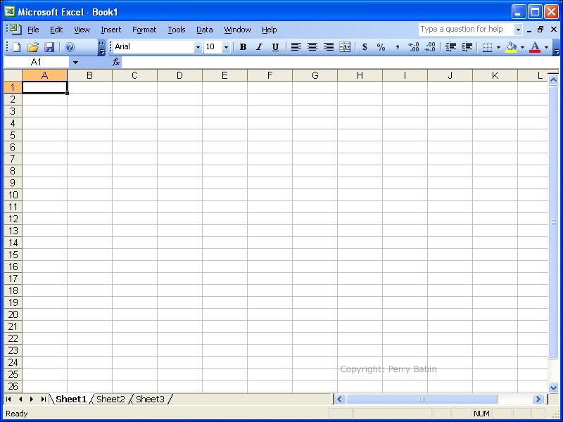
Overview:

Microsoft Excel is a spreadsheet programs that is primarily used for calculation and analysis. It is a very powerful tool. Here I will cover mainly the basic tools that the casual user may need. Below is s screenshot of a blank page. As you can see, there are rows (left/right) and columns (up/down) of cells. These cells will generally contain either numbers or formulas. The formulas can be as simple as adding the values of two cells.

Notes:

• If you click on a cell to select it, whatever you type will go into the cell and will overwrite the cell contents (if the cell was filled).
• After changing the contents of a cell, you can either hit the enter key or click on another cell to force the cell to accept the new content.
• If you hit the escape key before exiting the cell as described above, the content will revert to the previous values.
• If you have entered the new content, you can undo it by clicking the 'undo' arrow on the toolbar or going to EDIT >> UNDO.
• If you enter a cell by double-clicking it, you will have to highlight one or all of the characters to change them. To highlight, double-click in the open cell. You can also left-click and drag the mouse over the contents to highlight it.
• To copy the contents of a cell, select the cell(s) and click the 'copy' icon on the toolbar, select copy from the edit dialog box at the top of the page or RIGHT-click and select copy. After a cell is selected, the cell will be ringed by a dashed line. To past the contents to another cell, you can click the past icon on the toolbar, select paste from the edit dialog box or select paste from the right-click dialog box. You can also use the 'ctrl-C' and 'ctrl-V' keyboard shortcuts to copy and paste content.

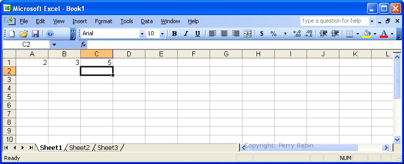
In the following image, you can see that there are three filled cells. The first two cells are filled with numbers. The third cell has a number in it but the cell is actually filled with a formula. The formula simply adds the first two cells.

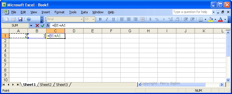
Here we see the formula as it really is. The formula adds the contents of column B row 1 to the contents of column A row 1. Note the letter/number combinations in the cell in column C (and also the field at above the spreadsheet). To let the cell know that the value you're about to enter is a formula instead of a value, you enter the '+' sign. Then you click on the first value you want to enter. After the first value is entered, you need to tell it what you want to do (add, subtract...) and you enter that function. After the function, you enter the next value. When you're finished, you hit the 'enter' key and the value will be displayed. If you enter something that can not be calculated, the spreadsheet will let you know.

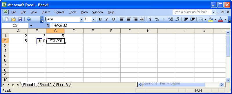
Below, we can see one such error. I tried to divide 5 by 0 and as soon as I hit enter, Excel showed me that there was a 'divide by zero' error.

In the example above, the values were all in adjacent cells. The values can be from any place on the sheet. Below, there are two non-adjacent cells multiplied together. Notice again that there is a 'plus' before the formula. When the formula cell is selected (by clicking it once or by using the arrow buttons), you can see the formula in the field above the spreadsheet. If you double-click the cell, the formula will be shown in the cell also.

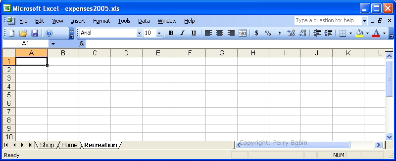
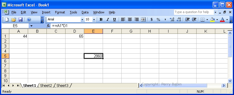If you look at the top of any of the images, you will see that the name of the file is 'book1'. The spreadsheets in Excel are known as workbooks. Look at them as individual ledgers or books. In each workbook, you can have many 'sheets' (near the bottom of the window). If you require multiple sheets, you should name them something that will allow you to instantly know what's on the sheet. Below, I've renamed the sheets and the workbook. To rename the sheet, double-click its tab. To enter values on any individual sheet, click on its tab. The selected sheet's tab will be white. All others will be dark.

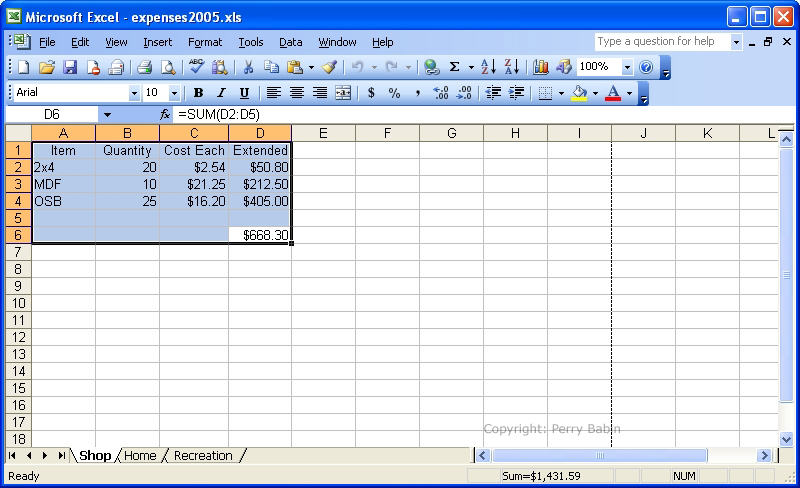
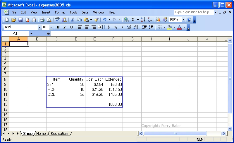
In the following image we have a lot of different things put together to serve a useful purpose. It's a list of building materials. As you can see, we have three rows of items (2x4s, MDF and OSB). We have the price of the individual items and the extended price. You already know how to do that. Adding the columns together is new (but simple). You click and select multiple cells (by dragging the mouse while the button is held down). To have a cell for the total, you have to select at least one extra cell. After the cells are selected, you simply press the 'sigma' button (the big funny looking 'E') on the toolbar.

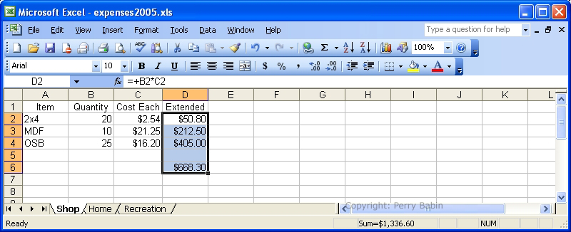In the image above, you can see a field in the lower left of the window. It says Sum=$1,336.60. This is the total of the highlighted items. You can use this to get a quick total of a list of items. Simply highlight all of the rows and/or columns that you want to total.

Setting Cell Size:
If the cell contents can not be shown in its entirety (as shown below) double-clicking the right-side divider of the cell letter bar sets the column size to fit the contents of all filled cells in that column. If you have one or two cells that have extraordinarily long content and they would make the rest of the cells too wide if you use the double-click method, you can simply drag the divider on the letter/number bar with the mouse until it's properly sized. You can resize the rows similarly by dragging the bottom of the corresponding divider on the number bar.

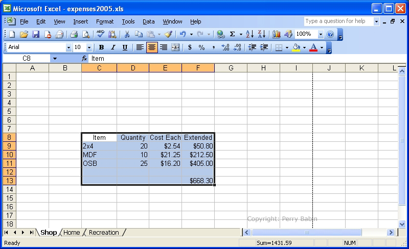
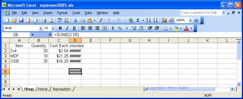Moving a Group of Cells:
If you need to move a group of cells, you can do it by clicking and dragging the mouse to highlight the desired cells. In the image below, I clicked on the bottom, right cell and dragged the mouse to the upper left cell. To move the selected cells, you move the mouse over the border of the selected cells. When the cursor changes from one arrow to 4 arrows, you click and drag the cells. The following image shows how the cursor looks when it's ready to move the cells.

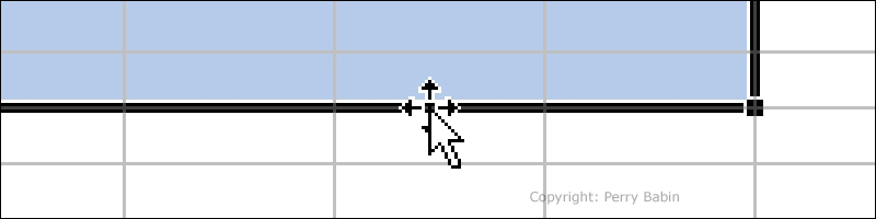The next two images show the original position with all of the cells highlighted and the results of the move.

Now, let's change the way the cells look. While the desired cells are highlighted, select FORMAT >> CELLS from the toolbar at the top of the page. In the dialog box, select the line style and color. Here we selected the double line and blue as the color. Then we clicked the 'outline' button to tell it to apply the formatting to the outer border of the selected set of cells.

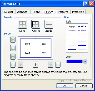Clicking Ok closed the dialog box and applied the formatting. Of course, this double blue outline is essentially useless but this is simply an example. You can apply formatting for the type of content (currency, scientific notation, general....), the color of the background or virtually any other property of the cells.

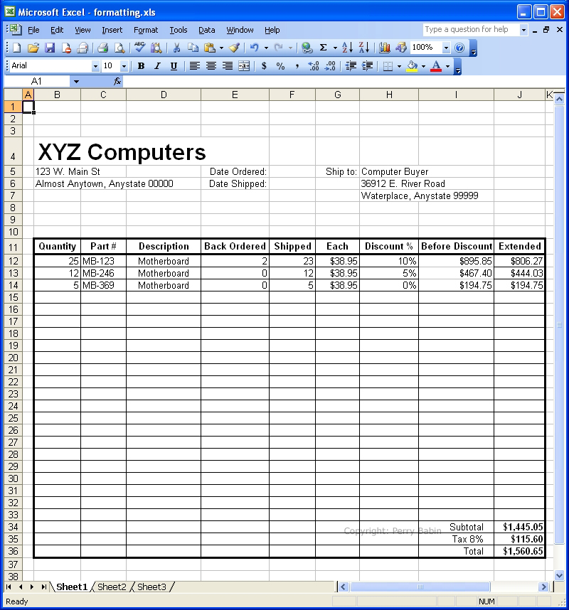
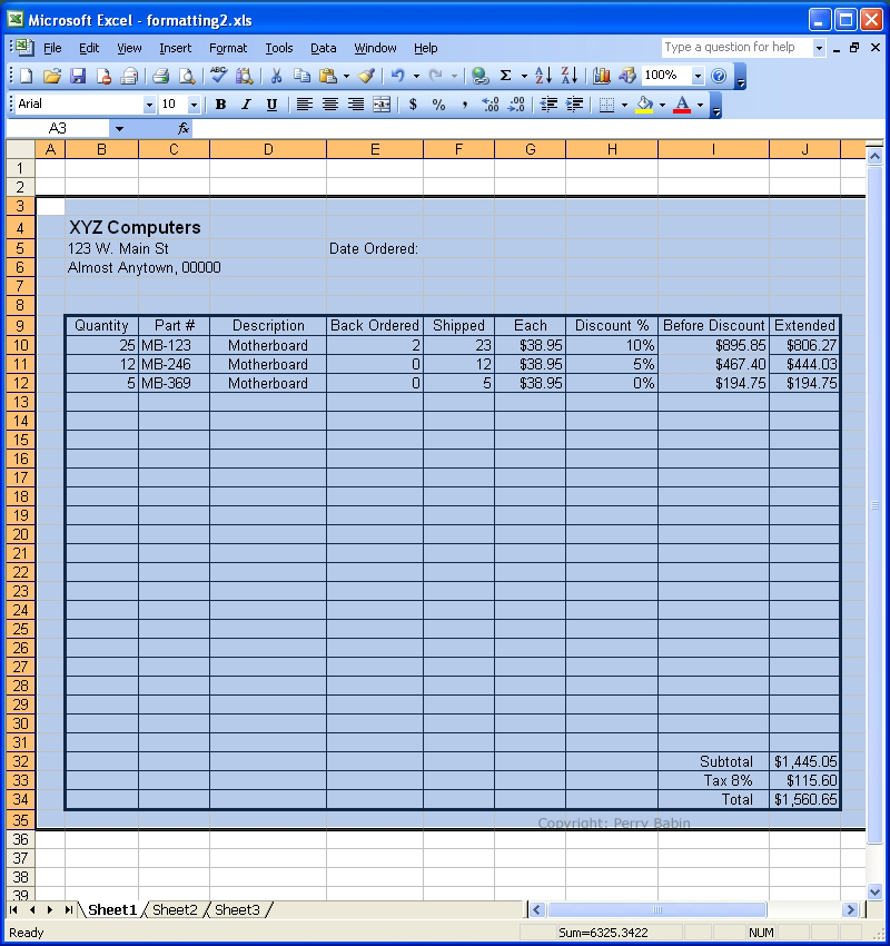
The following spreadsheet is closer to something that would be useful. The following formatting has been done:

• The Name of the business has been set larger than the rest of the text. To be precise, it's set to 24pt Arial Bold.
• The order and shipping date text has been aligned to the right.
• The border around the order form has been set to a bold black line.
• The internal cell lines have been set to something slightly bolder than the rest of the spreadsheet.
• The column label text has been centered both vertically as well as horizontally. It has also been set to a bold typeface.
• The subtotal, tax and total text have been aligned to the right but have an indent value of 1.
• The 'each', 'before discount' and 'extended' columns are formatted as currency. If you attempt to insert a dollar sign in the column, the spreadsheet will likely align it differently in the column. Formatting it as currency and allowing excel to add the dollar sign will generally work best.

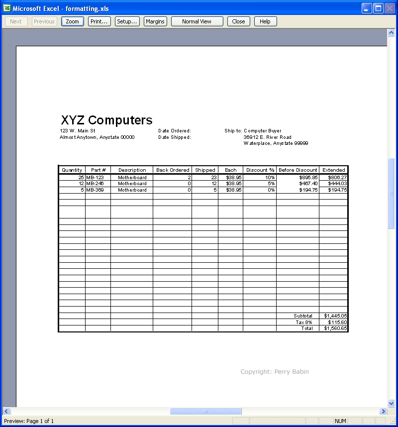
The view below is a 'print preview'. It shows you what you can expect when printed. As you can see, the majority of the cells are not shown.

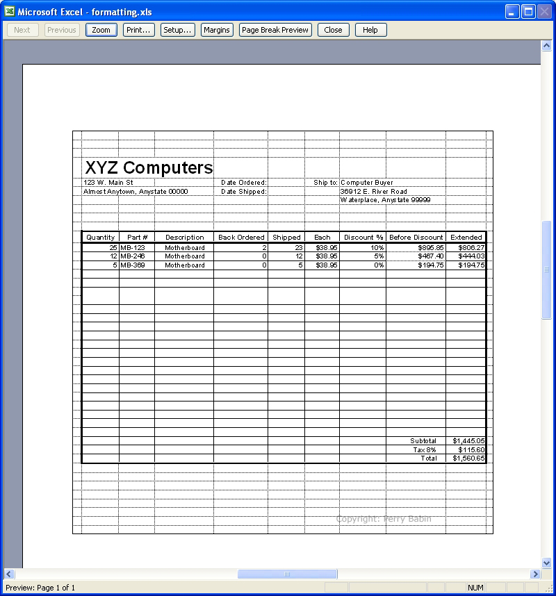
If you need to print something where all of the cells show, you can select that option in the page setup section. To get there... FILE >> PAGE SETUP >> select the SHEET tab and tell it you want to print the grid lines. This is what it looks like with the grid lines printed.

If you have Excel on your computer, right-click HERE and select SAVE TARGET AS then save it to a location you can find. When the download finishes (almost instantaneously), select OPEN. It should open in Excel. When in Excel, you can look at the various formulas and formatting and change them in any way you wish. If you simply click the link in Internet explorer, it will display the spreadsheet in the browser but it may not be editable won't give you all of the functions you have if you open it in Excel. If you simply click the link in Firefox, you will be asked if you wnat to open it in Excel. Of course, all of this assumes that you have Excel installed on your computer.

Inserting Graphics:
In some files, you will want to insert a logo or other graphic. Let's continue with this same file. Since we will be inserting a logo, we do not need the name as large as we have it above. To reduce it's size, we can simply select the cell where the text begins and reset the size by using the font size drop-down menu on the formatting toolbar. Here, I set it to a 12 point font.

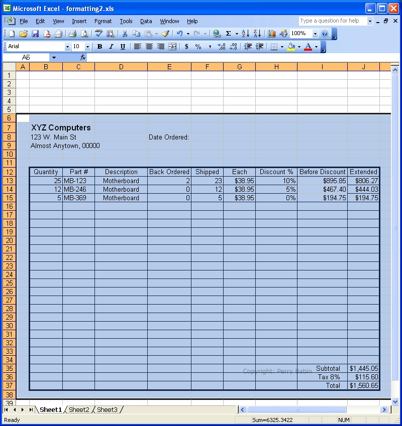
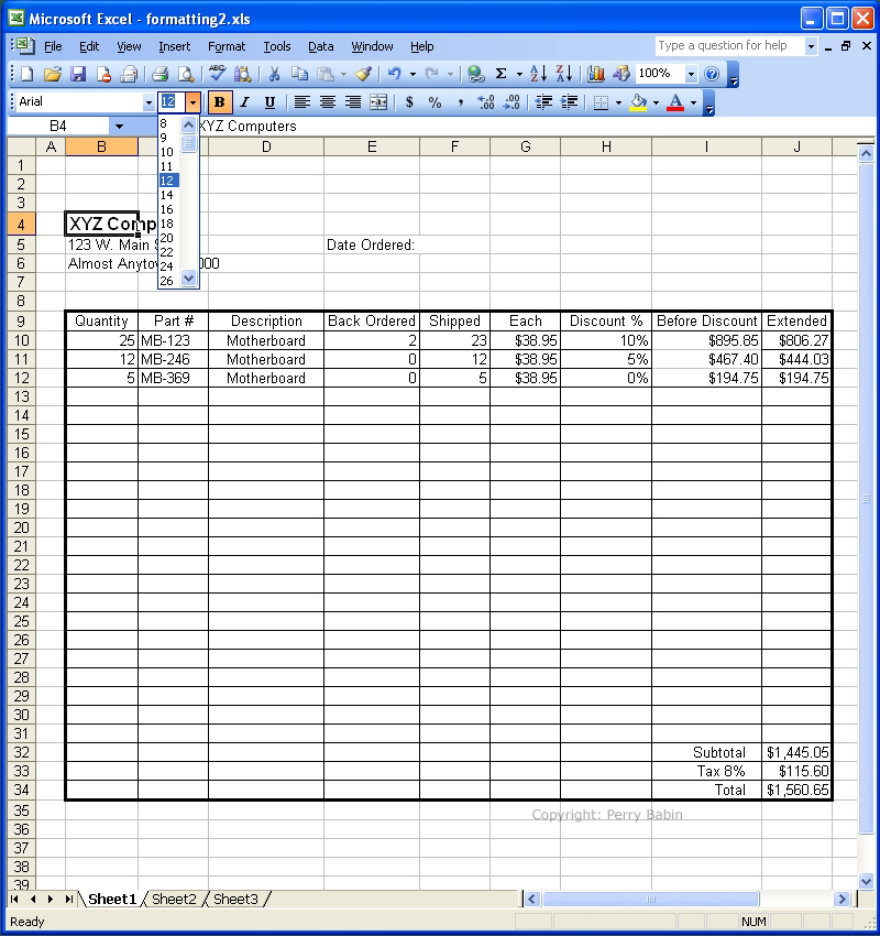Now, we need to move the current content down to make room for the image. As in a previous example, we have to highlight everything that we want to move. All that you 'really' need to highlight is the actual content but I highlighted one additional cell on all sides.

This is the content after we moved it.

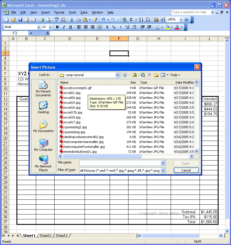
Below, we will INSERT a PICTURE from a FILE. Notice that cell F3 is highlighted. That's where the upper left corner of the image will be placed.

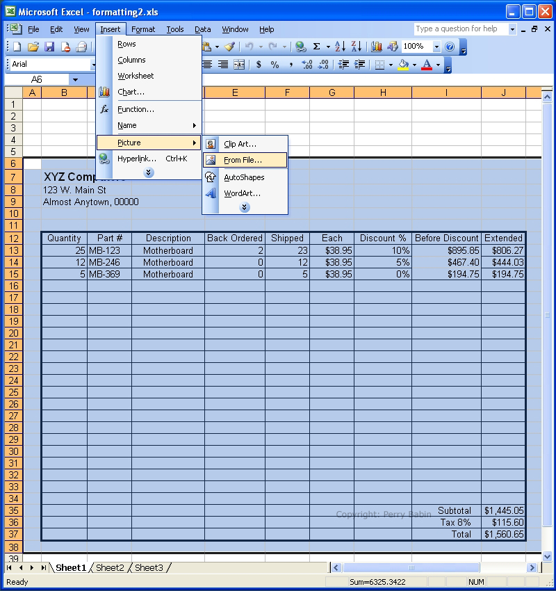Here, we simply select the image from the list of files. Of course, you have to know where the file has been saved. That's why you must pay attention to the folder name when you save a file. As we mentioned in the 'Working with Files' page, you should always save files to the same folder (or to the same group of organized folders).

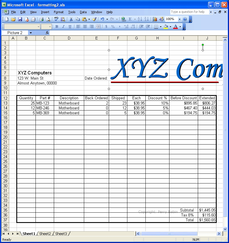
Now that the image has been inserted, it needs to be repositioned and resized. To move it, position the cursor over the image and drag it. To resize it without changing the aspect ratio you drag one of the corner handles (the little circles) until it is the desired size. If you wanted to change the aspect ratio (change either height OR width without changing the other), you would use one of the handles along the top or side of the image.

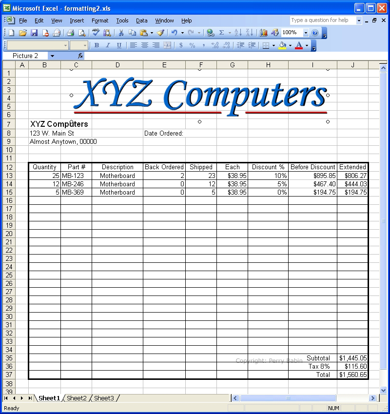
This is the finished product.

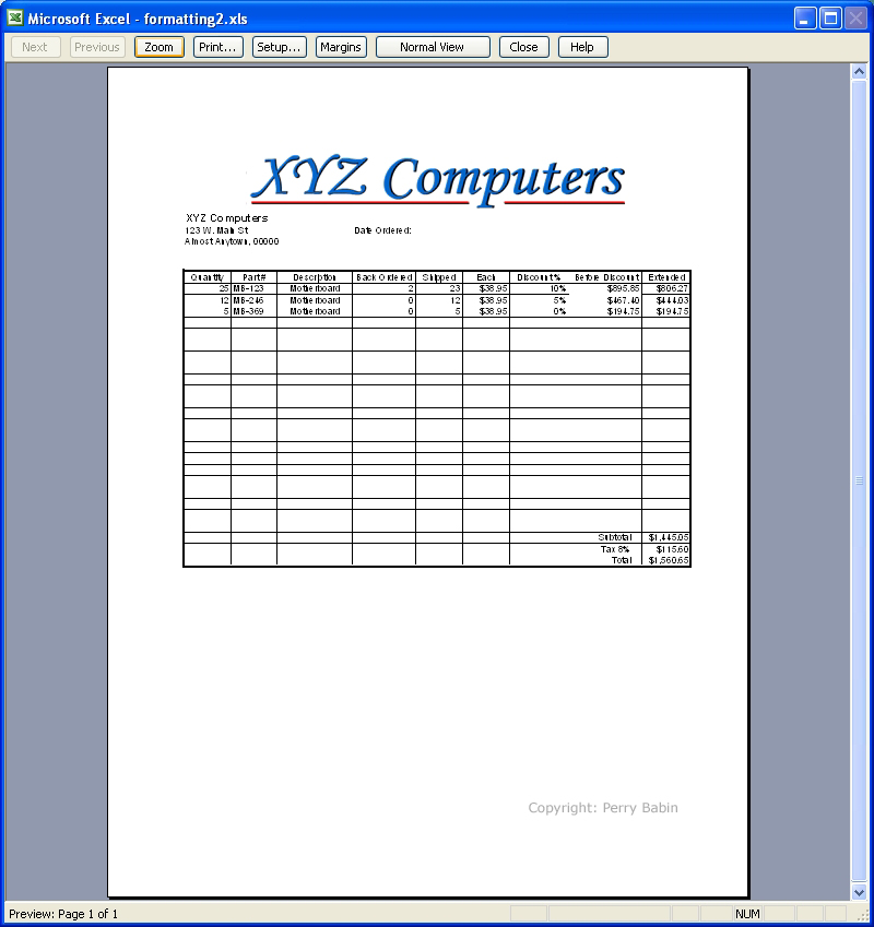
This is a 'print preview'. You will notice that some of the horizontal lines appear to be missing. This is due to the way the preview was rendered. When printed, all of the lines will appear as they should.

You May Be Interested in My Other Sites All Sorts of Stuff: This site was started for pages/information that didn't fit well on my other sites. It includes topics from backing up computer files to small engine repair to 3D graphics software to basic information on diabetes. Basic Macro Photography: This site introduces you to macro photography. Macro photography is nothing more than the photography of small objects. It can take quite a while to understand the limitations associated with this type of photography. Without help, people will struggle to get good images. Understanding what's possible and what's not possible makes the task much easier. If you need to photograph relatively small objects (6" in height/width down to a few thousandths of an inch), this site will help. Air Rifle Links and Demos: If you're interested in air rifles, this site will introduce you to the types of rifles available and many of the things you'll need to know to shoot accurately. It also touches on field target competition. There are links to some of the better sites and forums as well as a collection of interactive demos. Basic Car Audio Electronics: This site is for those who want to install or update their car stereo. It begins with the most basic electronics theory, progresses into basic transistor theory as well as covering virtually everything associated with car audio.